Convolution is one of the fundamental building block of Deep Neural Network (DNN) but sometimes, it can be extremely expensive to compute since it brings a lots of parameters and we are running risk of overfiting. This is where depthwise separable convolution can be used to reduce the total number of parameters, as a result, speed up convolution. This is a form of factorized convolutions which factorize a standard convolution into a depthwise convolution and a 1 x 1 convolution called a pointwise convolution.
What is Depthwise Separable Convolution?
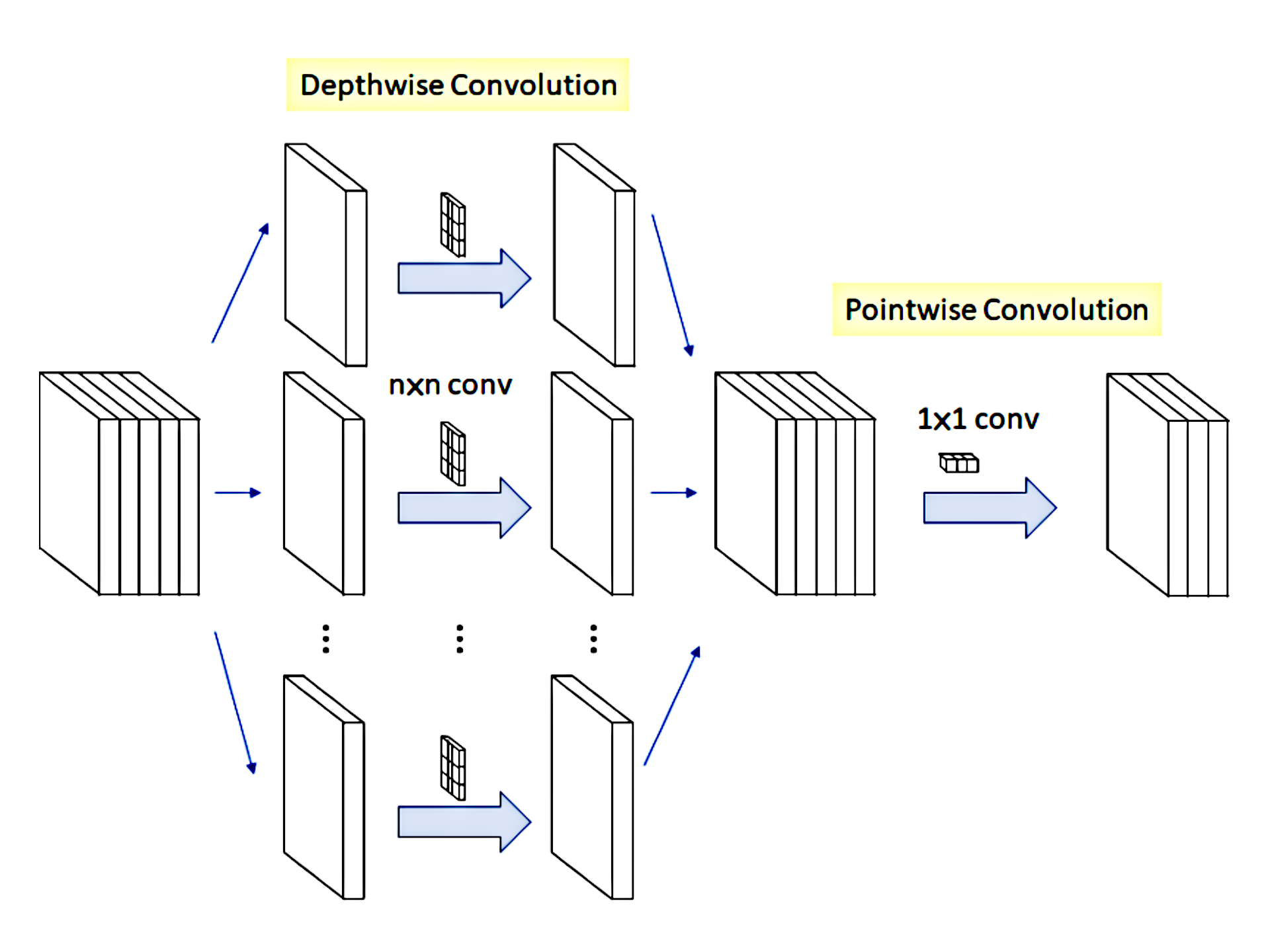
Depthwise separable convolution first use the depthwise convolution to applies a single filter to each input channel. Then the pointwise convolution is used to applies a 1 x 1 convolution to combine the outputs of the depthwise convolution. This differ from the standard convolution since it both filters and combines inputs into a new set of outputs in one step, thus more expensive in computation.
This depthwise separable convolution splits this into two layers, a separate layer for filtering and a separate layer for combining. This factorization has the effect of drastically reducing computation and model size.
Standard convolution
A standard convolution layer takes as input a $D_F \times D_F \times M$ feature map $F$ and produces a $D_F \times D_F \times N$ feature map $G$ where $D_F$ is the spatial width and height of a square input feature map (assume that the output feature map has the same spatial dimensions as the input and both feature maps are square), $M$ is the number of input channels (input depth), and $N$ is the number of output channel (output depth).
The standard convolutional layer is parameterized by convolution kernel $K$ of size $D_K \times D_K \times M \times N$ where $D_K$ is the spatial dimension of the kernel assumed to be square and $M$ is the number of input channels and $N$ is the number of output channels.
The output feature map for standard convolution assuming stride of one and padding is computed as: $$ G_{k,l,n} = \sum_{i,j,n} K_{i,j,m,n} \cdot F_{k+i-1,l+j-1,m} $$
standard convolutions have the computational cost of: $$ D_K \cdot D_K \cdot D_F \cdot D_F \cdot M \cdot N $$
That is, for one convolution operation, the number of multiplications is the number of elements in that kernel so that would be $D_K \times D_K \times M$ multiplications. But we slide this kernel over the input, we perform $D_K$ convolutions along the width and $D_K$ convolutions along the height and hence $D_K \times D_K$ convolutions over all. So the number of multiplications in the convolution of one kernel over the entire input $F$ is: $$ D_K \cdot D_K \cdot D_F \cdot D_F \cdot M $$ Now this is just one kernel but if we have $N$ such kernels which makes the absolute total number of multiplications become: $$ D_K \cdot D_K \cdot D_F \cdot D_F \cdot M \cdot N $$
Depthwise convolution
The standard convolution operation has the effect of filtering features based on the convolutional kernels and combining features in order to produce a new representation. The filtering and combination steps can be split into two steps via the use of factorized convolutions called depthwise separable convolutions for substantial reduction in computational cost.
Depthwise separable convolution are made up of two layers: depthwise convolution and pointwise convolutions. The depthwise convolution to apply a single filter per each input channel (input depth). Pointwise convolution, a simple 1 x 1 convolution, is then used to create a linear combination of the output of the depthwise layer.
First it uses depthwise convolutions to break the interaction between the number of output channels and the size of the kernel. Depthwise convolution with one filter per input channel (input depth) can be written as: $$ \hat G_{k,l,m} = \sum_{i,j} \hat K_{i,j,m} \cdot F_{k+i-1,l+j-1,m} $$
Where $\hat{K}$ is the depthwise convolutional kernel of size $D_K \times D_K \times M$ where the $m^{th}$ filter in $\hat{K}$ is applied to the $m^{th}$ channel in $F$ to produce the $m^{th}$ channel of the filtered output feature map $\hat{G}$.
Depthwise convolution has a computational cost of: $$ D_K \cdot D_K \cdot D_F \cdot D_F \cdot M $$
For depthwise convolution we use filters or kernels of shape $D_K \times D_K \times 1$ here it has a depth of one because this convolution is only applied to a channel, unlike standard convolution which is applied throughout the entire depth. Since we apply one kernel to a single input channel, we require $M$ such $D_K \times D_K \times 1$ over the entire input volume $F$ for each of these $M$ convolutions we end up with an output $D_F \times D_F \times 1$ in shape. Now stacking these outputs together we have an output volume of $G$ which is of shape $D_F \times D_F \times M$
Depthwise convolution is extremely efficient relative to standard convolution. However it only filters input channels, it does not combine them to create new features. So an additional layer that computes a linear combination of the output of depthwise convolution via 1 x 1 convolution is needed in order to generate these new features.
Pointwise convolution
Pointwise convolution involves performing the linear combination of each of these layers. Here the input is the volume of shape $D_F \times D_F \times M$, the filter has a shape of $1 \times 1 \times M$. This is basically a 1 x 1 convolution operation over all $M$ layers. The output this have the same input width and height as the input $D_F \times D_F$ for each filter. Assuming that we want to use some $N$ such filters, the output volume becomes $D_F \times D_F \times N$.
Now let’s take a look at the complexity of this convolution. We can split this into two parts as we have two phases. First we compute the number of multiplications in depthwise convolution. So here the kernels have a shape of $D_K \times D_K \times 1$ so the number of multiplications on one convolution operation is $D_K \times D_K$. When applied over the entire input channel this convolution is performed $D_F \times D_F$ number of times. So the total multiplications for the kernel over the input channels becomes $D_F \times D_F \times D_K \times D_K$. Now such multiplications are applies over all $M$ input channels. For each input channel we have a difference kernel and hence the total number of multiplications in the first phase that is depthwise convolution is $D_F \times D_F \times D_K \times D_K \times M$. Next we compute the number of multiplications in the second phase that is pointwise convolution. Here the kernels have a shape of $1 \times 1 \times M$ where M is the depth of the input volume. Hence the number of multiplications for one instance of convolution is $M$. This is applied to the entire output of the first phase which has a width and height of $D_F$ so the total number of multiplications for this kernel is $D_F \times D_F \times M$. So for some $N$ kernels we will have $N \times D_F \times D_F \times M$ such multiplications and thus the total number of multiplications in the depthwise convolution stage plus the number of multiplications in the pointwise convolution stage.
How exactly is this better?
Depthwise separable convolutions cost: $$ D_F \cdot D_F \cdot D_K \cdot D_K \cdot M + M \cdot N \cdot D_F \cdot D_F $$ By expressing convolution as a two step process of filtering and combining we get a reduction in computation of: $$ \frac{D_F \cdot D_F \cdot D_K \cdot D_K \cdot M + M \cdot N \cdot D_F \cdot D_F}{D_K \cdot D_K \cdot D_F \cdot D_F \cdot M \cdot N} \newline = \frac{D_K \cdot D_K + M}{D_K \cdot D_K \cdot N} \newline = \frac{1}{N} + \frac{1}{D^2_K} $$
To put this into perspective of how effective depthwise separable convolution is let us take an example. Consider the output features volume $N$ of 1024 and a kernel size 3, that is $D_K$ is equal to 3. Plugging these values into the relation we get 0.112. In other words depthwise separable convolution uses 8 to 9 times less computation than standard convolution.